Total derivative

In the mathematical field of differential calculus, the term total derivative has a number of closely related meanings.

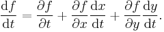
The total derivative (full derivative) of a function $f$ , of several variables, e.g., $t$ , $x$ , $y$ , etc., with respect to one of its input variables, e.g., $t$ , is different from its partial derivative ( $\partial$ ). Calculation of the total derivative of $f$ with respect to $t$ does not assume that the other arguments are constant while $t$ varies; instead, it allows the other arguments to depend on $t$ . The total derivative adds in these indirect dependencies to find the overall dependency of $f$ on $t$ . For example, the total derivative of $f(t,x,y)$ with respect to $t$ is

$\frac{\operatorname df}{\operatorname dt}=\frac{\partial f}{\partial t} %2B \frac{\partial f}{\partial x} \frac{\operatorname dx}{\operatorname dt} %2B \frac{\partial f}{\partial y} \frac{\operatorname dy}{\operatorname dt}.$

Consider multiplying both sides of the equation by the differential $\operatorname dt$ :

${\operatorname df}=\frac{\partial f}{\partial t}\operatorname dt %2B \frac{\partial f}{\partial x} \operatorname dx %2B \frac{\partial f}{\partial y} \operatorname dy.$

The result will be the differential change $\operatorname df$ in the function $f$ . Because $f$ depends on $t$ , some of that change will be due to the partial derivative of $f$ with respect to $t$ . However, some of that change will also be due to the partial derivatives of $f$ with respect to the variables $x$ and $y$ . So, the differential $\operatorname dt$ is applied to the total derivatives of $x$ and $y$ to find differentials $\operatorname dx$ and $\operatorname dy$ , which can then be used to find the contribution to $\operatorname df$ .

It refers to a differential operator such as

$\frac{\operatorname d}{\operatorname dx}= \frac{\partial }{\partial x}%2B\sum_{j=1}^k \frac{\operatorname dy_j}{\operatorname dx}\frac{\partial }{\partial y_j},$

which computes the total derivative of a function (with respect to x in this case).

It refers to the (total) differential df of a function, either in the traditional language of infinitesimals or the modern language of differential forms.

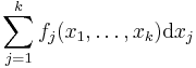
A differential of the form

$\sum_{j=1}^k f_j(x_1,\dots, x_k) \operatorname d{x_j}$

is called a total differential or an exact differential if it is the differential of a function. Again this can be interpreted infinitesimally, or by using differential forms and the exterior derivative.

It is another name for the derivative as a linear map, i.e., if f is a differentiable function from Rⁿ to R^m, then the (total) derivative (or differential) of f at x∈Rⁿ is the linear map from Rⁿ to R^m whose matrix is the Jacobian matrix of f at x.

It is a synonym for the gradient, which is essentially the derivative of a function from Rⁿ to R.

It is sometimes used as a synonym for the material derivative, $\frac{D\mathbf{u}}{Dt}$ , in fluid mechanics.

1 Differentiation with indirect dependencies
2 The total derivative via differentials
3 The total derivative as a linear map
4 Total differential equation
5 Application of the total differential to error estimation
6 References
7 External links

Differentiation with indirect dependencies

Suppose that f is a function of two variables, x and y. Normally these variables are assumed to be independent. However, in some situations they may be dependent on each other. For example y could be a function of x, constraining the domain of f to a curve in R². In this case the partial derivative of f with respect to x does not give the true rate of change of f with respect to changing x because changing x necessarily changes y. The total derivative takes such dependencies into account.

For example, suppose

$f(x,y)=xy$ .

The rate of change of f with respect to x is usually the partial derivative of f with respect to x; in this case,

$\frac{\partial f}{\partial x} = y$ .

However, if y depends on x, the partial derivative does not give the true rate of change of f as x changes because it holds y fixed.

Suppose we are constrained to the line

$y=x$

then

$f(x,y) = f(x,x) = x^2$ .

In that case, the total derivative of f with respect to x is

$\frac{\mathrm{d}f}{\mathrm{d}x} = 2 x$ .

Notice that this is not equal to the partial derivative:

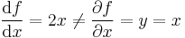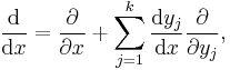
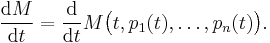
$\frac{\mathrm{d}f}{\mathrm{d}x} = 2 x \neq \frac{\partial f}{\partial x} = y = x$ .

While one can often perform substitutions to eliminate indirect dependencies, the chain rule provides for a more efficient and general technique. Suppose M(t, p₁, ..., p_n) is a function of time t and n variables $p_i$ which themselves depend on time. Then, the total time derivative of M is

${\operatorname{d}M \over \operatorname{d}t} = \frac{\operatorname d}{\operatorname d t} M \bigl(t, p_1(t), \ldots, p_n(t)\bigr).$

The chain rule for differentiating a function of several variables implies that

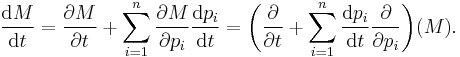
${\operatorname{d}M \over \operatorname{d}t} = \frac{\partial M}{\partial t} %2B \sum_{i=1}^n \frac{\partial M}{\partial p_i}\frac{\operatorname{d}p_i}{\operatorname{d}t} = \biggl(\frac{\partial}{\partial t} %2B \sum_{i=1}^n \frac{\operatorname{d}p_i}{\operatorname{d}t}\frac{\partial}{\partial p_i}\biggr)(M).$

This expression is often used in physics for a gauge transformation of the Lagrangian, as two Lagrangians that differ only by the total time derivative of a function of time and the n generalized coordinates lead to the same equations of motion. The operator in brackets (in the final expression) is also called the total derivative operator (with respect to t).

For example, the total derivative of f(x(t), y(t)) is

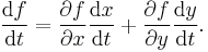
$\frac{\operatorname df}{\operatorname dt} = { \partial f \over \partial x}{\operatorname dx \over \operatorname dt }%2B{ \partial f \over \partial y}{\operatorname dy \over \operatorname dt }.$

Here there is no ∂f / ∂t term since f itself does not depend on the independent variable t directly.

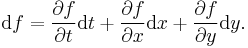
The total derivative via differentials

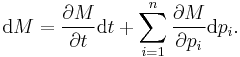
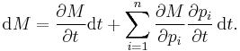
Differentials provide a simple way to understand the total derivative. For instance, suppose 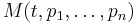$M(t,p_1,\dots,p_n)$ is a function of time t and n variables $p_i$ as in the previous section. Then, the differential of M is

$\operatorname d M = \frac{\partial M}{\partial t} \operatorname d t %2B \sum_{i=1}^n \frac{\partial M}{\partial p_i}\operatorname{d}p_i.$

This expression is often interpreted heuristically as a relation between infinitesimals. However, if the variables t and p_j are interpreted as functions, and $M(t,p_1,\dots,p_n)$ is interpreted to mean the composite of M with these functions, then the above expression makes perfect sense as an equality of differential 1-forms, and is immediate from the chain rule for the exterior derivative. The advantage of this point of view is that it takes into account arbitrary dependencies between the variables. For example, if $p_1^2=p_2 p_3$ then $2p_1\operatorname dp_1=p_3 \operatorname d p_2%2Bp_2\operatorname d p_3$ . In particular, if the variables p_j are all functions of t, as in the previous section, then

$\operatorname d M = \frac{\partial M}{\partial t} \operatorname d t %2B \sum_{i=1}^n \frac{\partial M}{\partial p_i}\frac{\partial p_i}{\partial t}\,\operatorname d t.$

The total derivative as a linear map

Let $U\subseteq \mathbb{R}^{n}$ be an open subset. Then a function $f:U\rightarrow \mathbb{R}^m$ is said to be (totally) differentiable at a point $p\in U$ , if there exists a linear map $\operatorname df_p:\mathbb{R}^n \rightarrow \mathbb{R}^m$ (also denoted D_pf or Df(p)) such that

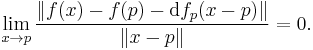
$\lim_{x\rightarrow p}\frac{\|f(x)-f(p)-\operatorname df_p(x-p)\|}{\|x-p\|}=0.$

The linear map $\operatorname d f_p$ is called the (total) derivative or (total) differential of $f$ at $p$ . A function is (totally) differentiable if its total derivative exists at every point in its domain.

Note that f is differentiable if and only if each of its components 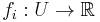$f_i:U\rightarrow \mathbb{R}$ is differentiable. For this it is necessary, but not sufficient, that the partial derivatives of each function f_j exist. However, if these partial derivatives exist and are continuous, then f is differentiable and its differential at any point is the linear map determined by the Jacobian matrix of partial derivatives at that point.

Total differential equation

Main article: Total differential equation

A total differential equation is a differential equation expressed in terms of total derivatives. Since the exterior derivative is a natural operator, in a sense that can be given a technical meaning, such equations are intrinsic and geometric.

Application of the total differential to error estimation

In measurement, the total differential is used in estimating the error Δf of a function f based on the errors Δx, Δy, ... of the parameters x, y, .... Assuming that the interval is short enough for the change to be approximately linear:

Δf(x) = f'(x) × Δx

and that all variables are independent, then for all variables,

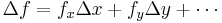
$\Delta f = f_x \Delta x %2B f_y \Delta y %2B \cdots$

This is because the derivative f_x with respect to the particular parameter x gives the sensitivity of the function f to a change in x, in particular the error Δx. As they are assumed to be independent, the analysis describes the worst-case scenario. The absolute values of the component errors are used, because after simple computation, the derivative may have a negative sign. From this principle the error rules of summation, multiplication etc. are derived, e.g.:

Let f(a, b) = a × b;

Δf = f_aΔa + f_bΔb; evaluating the derivatives

Δf = bΔa + aΔb; dividing by f, which is a × b

Δf/f = Δa/a + Δb/b

That is to say, in multiplication, the total relative error is the sum of the relative errors of the parameters.

References

A. D. Polyanin and V. F. Zaitsev, Handbook of Exact Solutions for Ordinary Differential Equations (2nd edition), Chapman & Hall/CRC Press, Boca Raton, 2003. ISBN 1-58488-297-2

From thesaurus.maths.org total derivative

External links

http://www.sv.vt.edu/classes/ESM4714/methods/df2D.html